Reference¶

Implementation of the standard load profiles

class oemof.demand.bdew.elec_slp.ElecSlp(year, seasons=None, holidays=None)[source]¶

Bases: object

Generate electrical standardized load profiles based on the BDEW method.

Parameters:

year (integer) – Year of the demand series.
Optional Parameters
——————-
seasons (dictionary) – Describing the time ranges for summer, winter and transition periods. The seasons dictionary will update the existing one, so only changed keys have to be defined. Make sure not to create time gaps. The “h0_dyn” will not work with changed seasons, so you have to use your own smoothing curve to create a “h0_dyn” profile.
holidays (dictionary or list) – The keys of the dictionary or the items of the list should be datetime objects of the days that are holidays.

all_load_profiles(time_df, holidays=None)[source]¶

create_bdew_load_profiles(dt_index, slp_types, holidays=None)[source]¶: Calculates the hourly electricity load profile in MWh/h of a region.

create_dynamic_h0_profile()[source]¶

property date_time_index¶

get_profile(ann_el_demand_per_sector)[source]¶

DEPRECATED: Use get_scaled_power_profiles() instead

Parameters:: ann_el_demand_per_sector (dictionary) – Key: sector, value: annual value
Returns:: pandas.DataFrame (Table with all profiles)

get_profiles(*args)[source]¶

Get all or the selected profiles. To select profiles you can pass: the name of the types as strings. The profiles are normalised to 1.

Try print(get_profiles().columns to get all valid types.

Returns:: pandas.DataFrame (Table with all or the selected profiles.)

Examples

>>> from oemof.demand import bdew
>>> e_slp = bdew.ElecSlp(year=2020)
>>> ", ".join(sorted(e_slp.get_profiles().columns))
'g0, g1, g2, g3, g4, g5, g6, h0, h0_dyn, l0, l1, l2'
>>> e_slp.get_profiles("h0", "g0").head()
                           h0        g0
2020-01-01 00:00:00  0.000017  0.000016
2020-01-01 00:15:00  0.000015  0.000015
2020-01-01 00:30:00  0.000014  0.000015
2020-01-01 00:45:00  0.000012  0.000014
2020-01-01 01:00:00  0.000012  0.000013

>>> e_slp.get_profiles("h0", "g0").sum()
h0    1.0
g0    1.0
dtype: float64

get_scaled_power_profiles(ann_el_demand_per_sector, conversion_factor=4)[source]¶

Get profiles scaled by there annual value. Each value represents the average power of an interval. Therefore, it is not possible to sum up the array. A conversion factor is used to calculate power units from energy units. By default the conversion factor is 4. As the interval of each profile is 15 minutes a conversion factor of 4 will convert energy units like Wh, kWh, MWh etc. to power units like W, kW, MW etc..

Parameters:

ann_el_demand_per_sector (dict) – The annual demand in an energy unit for each type.
conversion_factor (float) – Factor to convert the energy unit of the annual value to the power unit of each interval.

Returns:

pandas.DataFrame (Table with scaled profiles.)

Examples

>>> from oemof.demand import bdew
>>> e_slp = bdew.ElecSlp(year=2020)
>>> e_slp.get_scaled_power_profiles({"h0": 3000, "g0": 5000}).head()
                           g0        h0
2020-01-01 00:00:00  0.320338  0.202627
2020-01-01 00:15:00  0.305866  0.182365
2020-01-01 00:30:00  0.291590  0.164500
2020-01-01 00:45:00  0.278682  0.149633
2020-01-01 01:00:00  0.268122  0.138602
>>> cf = 4
>>> spp = e_slp.get_scaled_power_profiles({"h0": 3000, "g0": 5000},
...                                       conversion_factor=cf)
>>> spp.sum()
g0    20000.0
h0    12000.0
dtype: float64
>>> spp.div(cf).sum()
g0    5000.0
h0    3000.0
dtype: float64

get_scaled_profiles(ann_el_demand_per_sector)[source]¶

Get profiles scaled by there annual value.

Parameters:: ann_el_demand_per_sector (dict) – The annual demand in an energy unit for each type.
Returns:: pandas.DataFrame (Table with scaled profiles.)

Examples

>>> from oemof.demand import bdew
>>> e_slp = bdew.ElecSlp(year=2020)
>>> e_slp.get_scaled_profiles({"h0": 3000, "g0": 5000}).head()
                           g0        h0
2020-01-01 00:00:00  0.080084  0.050657
2020-01-01 00:15:00  0.076466  0.045591
2020-01-01 00:30:00  0.072897  0.041125
2020-01-01 00:45:00  0.069671  0.037408
2020-01-01 01:00:00  0.067030  0.034650

>>> e_slp.get_scaled_profiles({"h0": 3000, "g0": 5000}).sum()
g0    5000.0
h0    3000.0
dtype: float64

oemof.demand.bdew.elec_slp.dynamisation_function(timeindex: DatetimeIndex) → Series[source]¶

Use the dynamisation function of the BDEW to smoothen the seasonal edges. Functions resolution is daily.

$F_t = -3,92\cdot10^{-10} \cdot t^4 + 3,2\cdot10^{-7} \cdot t^3– 7,02\cdot10^{-5}\cdot t^2 + 2,1\cdot10^{-3} \cdot t + 1,24$

With t the day of the year as a decimal number.

Implementation of the bdew heat load profiles

class oemof.demand.bdew.heat_building.HeatBuilding(df_index, **kwargs)[source]¶

Bases: object

Parameters:

year (int) – year for which the profile is created

Variables:

datapath (string) – path to the bdew basic data files (csv)
temperature (pandas.Series) – Series containing hourly temperature data
annual_heat_demand (float) – annual heat demand of building in kWh
building_class (int) – class of building according to bdew classification: possible numbers for EFH and MFH are: 1 - 11. Possible numbers for non-residential buildings are: 0.
shlp_type (string) – type of standardized heat load profile according to bdew possible types are: GMF, GPD, GHD, GWA, GGB, EFH, GKO, MFH, GBD, GBA, GMK, GBH, GGA, GHA
wind_class (int) – wind classification for building location (0=not windy or 1=windy)
ww_incl (boolean) – decider whether warm water load is included in the heat load profile
ww_only (boolean) – if true, only warm water load is included in the heat load profile

get_bdew_profile()[source]¶: Calculation of the hourly heat demand using the bdew-equations

get_normalized_bdew_profile()[source]¶: Calculation of the normalized hourly heat demand

get_sf_values(filename='shlp_hour_factors.csv')[source]¶

Determine the h-values

Parameters:: filename (string) – name of file where sigmoid factors are stored

get_sigmoid_parameters(filename='shlp_sigmoid_factors.csv')[source]¶

Retrieve the sigmoid parameters from csv-files

Parameters:: filename (string) – name of file where sigmoid factors are stored

get_temperature_interval()[source]¶: Appoints the corresponding temperature interval to each temperature in the temperature vector.

get_weekday_parameters(filename='shlp_weekday_factors.csv')[source]¶

Retrieve the weekday parameter from csv-file

Parameters:: filename (string) – name of file where sigmoid factors are stored

weighted_temperature(how='geometric_series')[source]¶

A new temperature vector is generated containing a multi-day average temperature as needed in the load profile function.

Parameters:: how (string) – string which type to return (“geometric_series” or “mean”)

Notes

Equation for the mathematical series of the average temperature [1]:

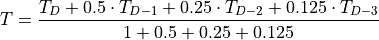
$T=\frac{T_{D}+0.5\cdot T_{D-1}+0.25\cdot T_{D-2}+ 0.125\cdot T_{D-3}}{1+0.5+0.25+0.125}$

with $T_D$ = Average temperature on the present day: $T_{D-i}$ = Average temperature on the day - i

References

Implementation of industrial step load profiles.

class oemof.demand.particular_profiles.IndustrialLoadProfile(dt_index, holidays=None, holiday_is_sunday=False)[source]¶

Bases: object

Generate an industrial heat or electricity load profile.

simple_profile(annual_demand, **kwargs)[source]¶

Create industrial step load profile.

Parameters:

annual_demand (float) – Total demand over the period given upon initialisation of IndustrialLoadProfile through parameter dt_index. This is actually only the annual demand, if an entire year was given.

Other Parameters:

am (datetime.time) – Defines the beginning of the workday. Times between am and pm, including the start and end time defined by am and pm, are assigned “day” factors from profile_factors. Other times are assigned “night” factors. Default: 7 a.m.
pm (datetime.time) – Defines the end of the workday. Times between am and pm, including the start and end time defined by am and pm, are assigned “day” factors from profile_factors. Other times are assigned “night” factors. Default: 11:30 p.m.
week (list(int)) – List of weekdays, where 1 corresponds to Monday, 2 to Tuesday, etc. Weekdays are assigned “week” factors from profile_factors. Default: [1, 2, 3, 4, 5].
weekend (list(int)) – List of weekend days, where 1 corresponds to Monday, 2 to Tuesday, etc. Weekend days are assigned “weekend” factors from profile_factors. Default: [6, 7].
holiday (list(int)) – List of holiday days. Holidays given upon initialisation of the IndustrialLoadProfile object are tagged with weekday 0 if holiday_is_sunday is set to False, wherefore the default for this parameter is [0]. Holidays are assigned “holiday” factors from profile_factors. Default: [0].
profile_factors (dict) – Dictionary with load profile scaling factors for night and day of weekdays, weekend days and holidays. The dictionary must have the same form as the dictionary given as the default value. Default:
```
{
    "week": {"day": 0.8, "night": 0.6},
    "weekend": {"day": 0.9, "night": 0.7},
    "holiday": {"day": 0.9, "night": 0.7},
}
```

Returns:

pd.Series – Series with demand per time step (unit depends on the unit the annual_demand was provided with). Index is a DatetimeIndex containing all time steps the IndustrialLoadProfile was initialised with.

The region module combines profiles from VDI 4655 for heat and power demand of houses within one region.

This is an implementation of the calculation of load profiles defined in the German VDI 4655.

VDI 4655

Reference load profiles of single-family and multi-family houses for the use of CHP systems

May 2008 (ICS 91.140.10)

Verein Deutscher Ingenieure e.V.

VDI Standards Department

VDI-Platz 1, 40468 Duesseldorf, Germany

Reproduced with the kind permission of the Verein Deutscher Ingenieure e.V.

Notes

This script creates full year energy demand time series of domestic buildings for use in simulations. This is achieved by an implementation of the VDI 4655, which gives sample energy demands for a number of typical days (‘Typtage’). The energy demand contains heating, hot water and electricity.

For a given year, the typical days can be matched to the actual calendar days, based on the following conditions: - Season: summer, winter or transition - Day: weekday or sunday (Or holiday, which counts as sunday) - Cloud coverage: cloudy or not cloudy - House type: single-family houses or multi-family houses (EFH or MFH)

class oemof.demand.vdi.regions.Climate(temperature=None, cloud_coverage=None, energy_factors=None)[source]¶

Bases: object

Climate object for VDI time series.

Parameters:

temperature (iterable of numbers) – The ambient temperature in the area as daily mean values. The number of values must equal 365 or 366 for a leap year. Use the TRY data if no temperature data is available.
cloud_coverage (iterable of numbers) – The cloud coverage in the area as daily mean values. The number of values must equal 365 or 366 for a leap year.

check_attributes()[source]¶

from_try_data(try_region, hoy=8760)[source]¶

class oemof.demand.vdi.regions.Region(year, climate, seasons=None, holidays=None, houses=None, resample_rule=None, zero_summer_heat_demand=False)[source]¶

Bases: object

Define region-dependent boundary conditions for the load profiles.

After adding houses to the region, the load profiles for each house can be generated.

Parameters:

year (int) – Year of the profile.
seasons (dict (optional)) – The times of the seasons if fixed seasons are used. In the VDI norm seasons are defined by the daily average temperature: Winter below 5 degree Celsius, Spring between 5 and 15 degree Celsius and summer above 15 degree Celsius.
holidays (dict or list (optional)) – In case of a dictionary the keys are datetime objects and the values are strings with the name of the holiday. Otherwise a list of datetime objects should be passed.
houses (list (optional)) – A list of dictionaries in which each house is defined the dictionary need to have the following keys.
resample_rule (str (optional)) – Time interval to resample the profile e.g. 1h (1 hour) or 15min. The value will be passed to the pandas resample method.
zero_summer_heat_demand (bool (optional)) – Set heat demand on all summer days to zero. Per default, multi-family houses have a small heat demand even in summer. (This is not part of VDI 4655)

add_houses(houses)[source]¶

Add houses to the region object.

Parameters:

houses (list) – A list of dictionaries that describes the houses.

Required parameters for each house:

name: Unique identifier for the house
house_type: Either “EFH” (single-family) or “MFH” (multi-family)
N_Pers: Number of persons, up to 12 (relevant for EFH)
N_WE: Number of apartments, up to 40 (relevant for MFH)
Q_Heiz_a: Annual heating demand in kWh
Q_TWW_a: Annual hot water demand in kWh
W_a: Annual electricity demand in kWh

Optional:

summer_temperature_limit: Temperature threshold for summer season (default: 15°C)
winter_temperature_limit: Temperature threshold for winter season (default: 5°C)

get_daily_energy_demand_houses(tl)[source]¶: Determine the houses’ energy demand values for each ‘typtag’.

Note

“The factors F_el_TT and F_TWW_TT are negative in some cases as they represent a variation from a one-year average. The values for the daily demand for electrical energy, W_TT, and DHW energy, Q_TWW_TT, usually remain positive. It is only in individual cases that the calculation for the typical-day category SWX can yield a negative value of the DHW demand. In that case, assume F_TWW_SWX = 0.” (VDI 4655, page 16)

This occurs when N_Pers or N_WE are larger than their allowed maximum of 12 persons (for single-family houses) and 40 apartments (for multi-family houses).

get_load_curve_houses()[source]¶

Generate time series of energy demand values for all houses.

This method calculates the energy demands heating, hot water, and electricity for each house in the region based on the VDI 4655 typical day profiles. The calculation uses daily energy demands and typical load profiles, which are combined to create a full year time series for each house and energy type.

The resulting time series are normalized to match the annual energy demands specified in the house parameters (Q_Heiz_a, Q_TWW_a, W_a).

Returns:

pandas.DataFrame – MultiIndex DataFrame with the following structure:

Index: DatetimeIndex with the time steps
Columns: MultiIndex with levels
- name: House identifier
- house_type: Either “EFH” or “MFH”
- energy: Energy type (“Q_Heiz_TT”, “Q_TWW_TT”, or “W_TT”)
Values: Energy demand in kWh per time step

Read DWD TRY (test reference year) data.

oemof.demand.vdi.dwd_try.find_try_region(longitude, latitude)[source]¶

Find the DWD TRY region by coordinates.

Note

Latitude and longitude must be provided in the coordinate reference system EPSG:4326.
The packages geopandas and shapely need to be installed to use this function.

Parameters:

longitude (float)
latitude (float)

Returns:

DWD TRY region number (int)

Raises:

ImportError – If geopandas or shapely are not installed

oemof.demand.vdi.dwd_try.read_dwd_weather_file(weather_file_path)[source]¶

Read and parse DWD test reference year (TRY) weather data files.

This function reads TRY weather data files published by the German Weather Service (Deutscher Wetterdienst, DWD) and extracts temperature and cloud cover data.

The 2016 DWD weather files can be obtained from: https://kunden.dwd.de/obt/ (registration required)

Parameters:

weather_file_path (str, optional) – Path to a TRY weather file. The file must follow the DWD format from 2010 or 2016. If None, a default file for the given try_region will be used.

Returns:

pandas.DataFrame – DataFrame with hourly weather data

Raises:

TypeError – If the weather file does not follow the expected DWD format
FileNotFoundError – If the weather file cannot be found

Reference¶

Table of Contents

This Page